Anomaly Detection with MEMS Vibration Sensors and Machine Learning - Part 3/3 Bearing Damage Detection

This is the third part in a three-part series.
Part 1: Sensors in a Waste Processing Plant
Part 2: Anomaly Detection with Autoencoders
Real-world Vibratory Screen Data
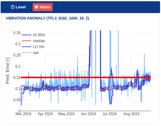
Figure 23 shows the autoencoder loss of a vibratory screen, based on 4,400
measurements (3x8192 samples/meas) collected from a triax MEMS sensor between
February and August 2024 on a vibratory screen as depicted in Figure 5
(see Part 1).
The monitored period spans a period of 7 months of measurements and
telemetry data with an estimated 70% of remaining battery capacity.
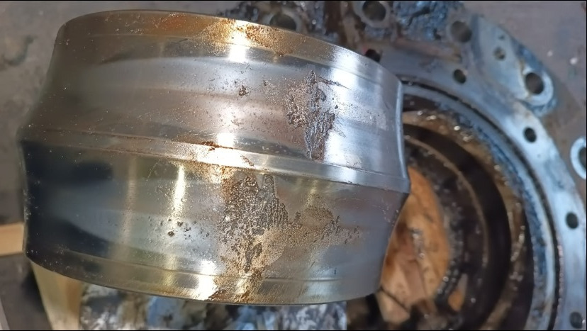
The historical data reveals the progression of a bearing fault over time:
- Training data from February to March (600 measurements)
- Signs of initial damage become detectable around March 24 (T-70d)
- Further deterioration (stage-3) from May 22 onwards (T-11d)
- Critical damage (stage-4 bearing fault) on June 2 (T)
- The bearing was replaced on June 17 (T+15d)
Beyond the bearing failure, the data also shows a new increase in the anomaly level on August 8 (far right side fig. 23). This rise has been confirmed to be caused by a bent shaft, which was scheduled for replacement during the upcoming maintenance cycle.

Limitations of RMS-only sensors
Figure 25 illustrates the lack of sensitivity of an RMS-only sensor for bearing fault detection. Due to the in-band process noise, the fault’s energy stays undetectable until the very last stages, when it rises above the total integrated noise floor. Relying only on time-domain data or simple RMS thresholds is thus insufficient for early fault warnings.
Spectral Heatmap
To review and understand the ML results, we introduce the spectral heatmap. In this plot, the horizontal x-axis represents measurement date, and the vertical slices (y-axis) represents the frequency spectrum of 1 single measurement (z-axis). Similar to the STFT, the energy in the spectrum is represented by a color map, with dark blue indicating the lowest magnitude and yellow the highest peaks.
Upper part of the spectrum
In the spectrum above 300Hz (bin >1500), we can observe some early stage
indicators of an upcoming change in the behaviour of the machine. The first
warning (‘initial damage’) appears around 10 weeks before the critical damage
of the bearing, then it disappears temperorarily because of routine
maintainance.
Around 11 days before the bearing failure it appears again. In the final stage of the bearing damage, we can see the fault spectrum spread out over all frequency bands, which is the well-known indicator for stage-4 bearing damage.
Lower part of the spectrum
Figure 24 also shows that most of the process noise is concentrated around
the fundamental drive frequency and its harmonics. For example, bin 500
(97Hz) shows the process noise modulated onto the 2nd harmonic (asynchronous
motor at mains frequency of 50Hz with 3% slip).
In the lower part of the spectrum, the harmonics originate partially from the inevitable slight imbalance combined with the very rigid structure of the screen itself and partially due to the nonlinear behaviour of the screen’s separator structures. Apart from the static load on the bearing, the high forces due to the rigid bearing and the dynamic imbalance are the main cause of a reduced service life of the eccentric shaft bearing.
For an in-depth analysis, see
[researchgate.net]
:

Mitigation of False Positives
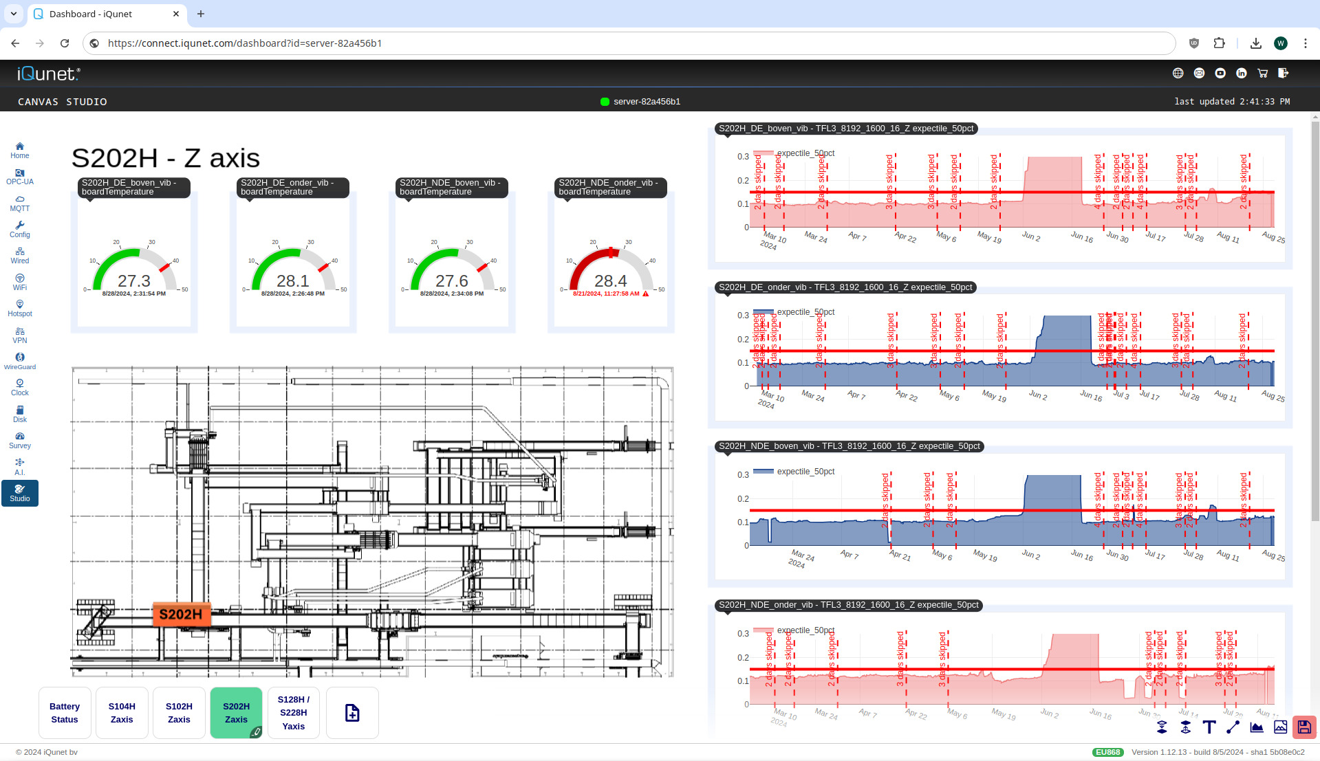
While the spectral heatmap provides detailed insights into the operational behavior of the vibratory screen, visually inspecting a heatmap for each sensor is impractical on a daily basis for more than a few sensor nodes.
The key advantage of the “STFT + autoencoder + loss function” approach is its ability to project complex sensor signals onto a single numeric “anomaly score” via a nonlinear mapping.
The anomaly score then allows us to use a simple, temperature-like threshold based on historical anomaly values. This eliminates the need to manually set alarm levels for each individual frequency subrange. This is especially true for equipment that comes with little a-priori information, such as small ubiquitous equipment like pumps, conveyor belts, or fans.

[Click image to enlarge]
To minimize false alarms, the output of the loss detector is smoothed using a rolling window quantile estimator before being compared to the threshold. A lower quantile with a larger window reduces the likelihood of false alarms but slows response time. Conversely, a higher quantile increases sensitivity at the expense of more false positives. Using multiple quantiles with a single threshold provides alarms with varying severity levels.

When the alarm is triggered, the anomaly score continues to provide insights into the stability of the anomaly: we can now see of how rapidly the machine is deviating from its operational baseline. It provides useful data for how fast an intervention must be planned.
Conclusion
Wireless vibration sensors combined with machine learning provide a powerful solution for day-to-day anomaly detection in industrial screens. By continuously monitoring machine behavior and processing data through deep-learning ML models, emerging random faults can be detected before they become catastrophic. Leveraging the strength of big data tips the scale in favor of MEMS technology, even with some reduced sensitivity/bandwidth compared to piezo sensors.
This predictive approach minimizes unplanned downtime, and allows to align repairs with the scheduled maintenance. The ability to automatically detect complex issues without relying on manual inspections or preset thresholds highlights the potential of integrating machine learning into industrial maintenance strategies, bringing the required level of understanding from expert vibration analist to anyone with a good technical background.
For more detailed technical insights and support, explore our documentation and case studies, or contact our support team.


