Anomaly Detection with MEMS Vibration Sensors and Machine Learning - Part 2/3 Deep Learning
This is the second part in a three-part series.
Part 1: Sensors in a Waste Processing Plant
Part 3: Real-world Vibratory Screen Data
Sensor Data Processing and Machine Learning
The MEMS-based wireless vibration sensors (IVIB161010-ACC3-016) gather detailed, day-to-day data containing info about the vibratory screen’s behavior (see part 1).
Each sensor captures three-axis vibration snapshots every 20 minutes (configurable) at a sampling rate of 3200Hz (also configurable). A measurement, consisting of up to 25,000 samples, is wirelessly transferred to a central edge server equipped with an embedded historian database.
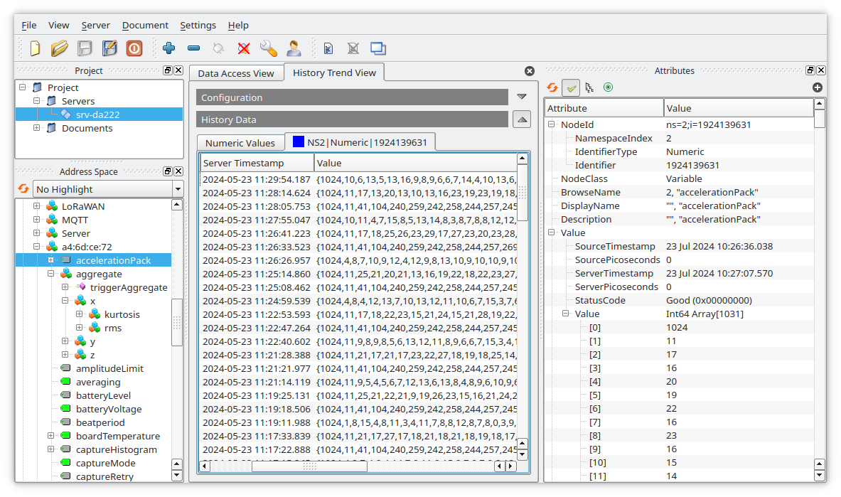
(image: UaExpert OPC-UA client. [link])
The iQunet edge server includes a TensorFlow processor for machine learning inference, along with a customizable dashboard, making it a complete standalone solution. For compatibility with third-party applications, the software also comes with an OPC-UA server and MQTT publishing client, enabling real-time visualization on the most common SCADA platforms (Kepware, Ignition, Siemens SIMATIC, etc.) and cloud-based IoT systems.
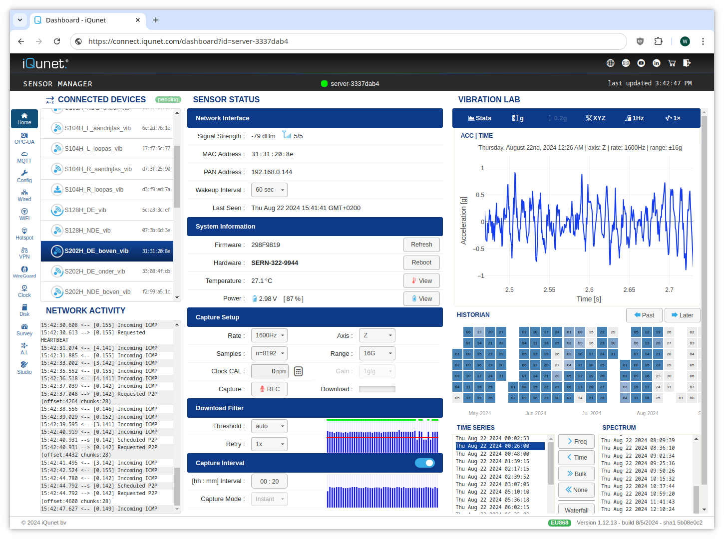
(click to enlarge).
From Raw Data to Actionable Insights
The raw vibration data (i.e. acceleration time series vectors) collected by the sensors undergoes several preprocessing steps to extract several aggregate and more complex signal transformations, discussed below:
Prefiltering, Data Streams and Domains
Prefiltering
While some types of piezo sensors can directly generate high dynamic range
velocity signals at very low frequencies using a charge-mode amplifier, most
sensors types are acceleration-based. This means that the output needs to be
integrated from m/s2 to m/s to derive the velocity signal.
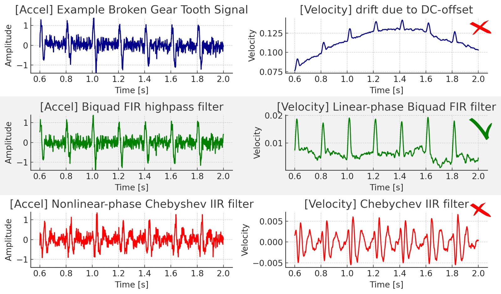
MEMS sensors are no different in this matter and are also acceleration based. Their output signal contains a large dc-signal (the gravitation component) which needs to be removed before the conversion to velocity.
Expert Insights
Filtering is a complex mathematical process, similar to the preamp stabilization time in piezo sensors. It is important to ensure that the high rejection ratio of a highpass filter does not introduce ripple or phase errors, as these can distort the time-domain signal and also cause significant drift when integrating from acceleration to velocity. Linear phase-filters, such as multi-stage digital FIR filters, are typically used to address these challenges.
Data Streams
Once the dc-offset is removed, the data is converted into several useful
information streams in the edge server, including:
- Acceleration and velocity
- RMS and Kurtosis aggregate values
- Time and frequency domain views
These are some of the basic tools used by vibration experts to determine
the state of the machine, and in more advance cases, also the origin of a
fault, such as a loose mount or a bearing fault.
Other tools, such as enveloping demodulation, further postprocess the signal,
primarily to represent the same data in a format or domain that is more
easily understood by the human eye.
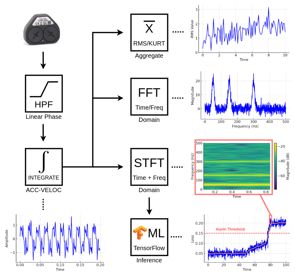
However, this blog post focuses on the automated detection of anomalies and faults using machine learning techniques. It’s important to understand that the specific formats in which vibration data is represented are less critical for deep-learning models, as these tools will ‘learn’ the optimal latent representation of the data during the training phase.
Time and Frequency Domain
So why would a vibration expert use both the time and frequency views?
Although they represent the same underlying information, each domain has its
advantages when it comes to detecting specific signal patterns.
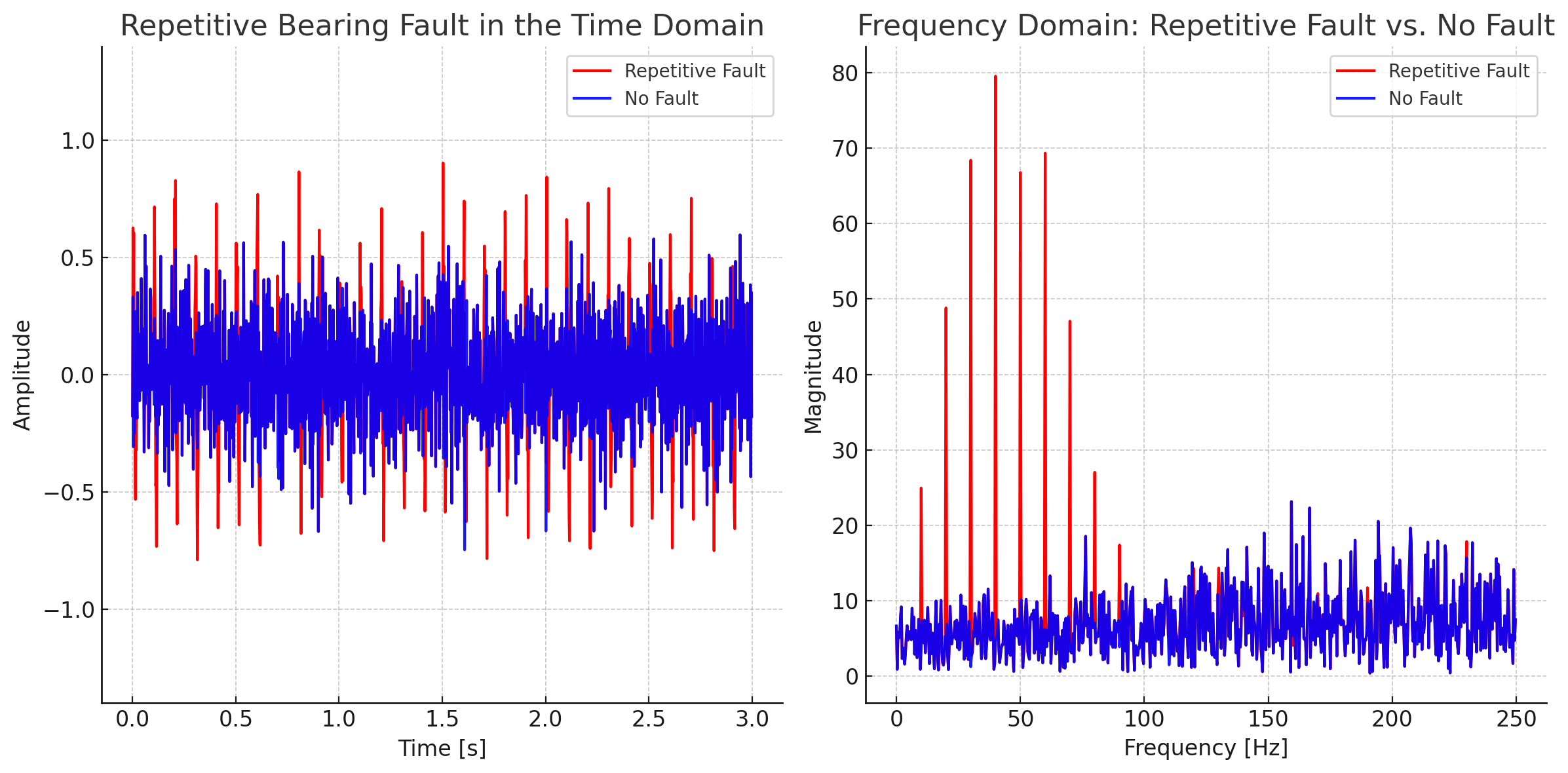
For instance, one-time or repetitive transient events in the signal (e.g. a mechanical impulse) are easily identified in the time domain, where their energy is concentrated in a short interval. However, in the frequency domain, the same short event merely appear as a slight wideband bump above the noise floor, making them difficult to detect.

Early-stage bearing faults (stage 1/2) are most effectively detected with piezo sensors at ultrasonic frequencies, where the noise floor is lower and thus more favorable to detect unusual patterns in the spectrum.
However for repetitive impulses, energy concentrates around key fault
frequencies(*), such as BPFI and BPFO (stage 2/3). These which are well
within the capabilities of modern MEMS sensors. Nevertheless, capturing
sufficient impulses to rise above the noise floor is essential. Extended
measurements, however, may still pose challenges for wireless sensors due
to their data (transfer) and battery constraints.
(*) More info here:
[reliabilityconnect.com]
.
Sometimes you need a cost-effective solution for a real-world application outside the lab. MEMS sensors can offer the middle ground between the ultimate monitoring equipment and nothing. The amount of data that continuous monitoring offers often makes the choice for MEMS more suitable than periodic manual inspections.
The above consideration is important for understanding why we use the Short-Time Fourier Transform (STFT) when feeding data into the machine learning algorithm. The STFT allows us to represent the sensor signal in both the time- and frequency-domain simultaneously. By doing so, we capture all relevant information (for the sake of simplicity, we exclude phase information here) and ensure that the signal power of various fault patterns, whether time-based or frequency-based, remains concentrated and is more easily detected.
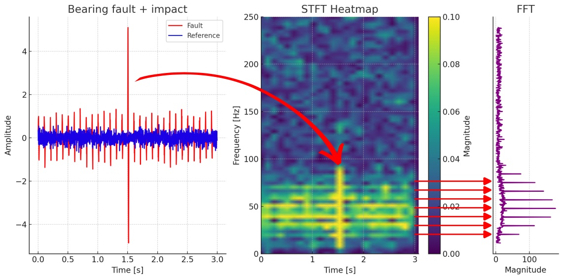
While it is very possible for a machine learning algorithm to perform domain transforms internally, this approach would require a significant portion of the model structure (specifically, the convolutional layers) to handle these transforms. This would complicate the training phase as it would also take considerable training time to tune the ML model parameters to ‘invent’ these transforms.

By using the STFT as a fixed preprocessing step, we effectively offload this task and provide the ML algorithm with a rich feature input that combines the strengths of both domains. In this sense, the STFT acts as a pre-trained, fixed component of the machine learning model itself, simplifying the detection process and reducing the training time for each sensor node.
Challenges with Manual Analysis and Traditional Methods
Linking specific fault patterns to their root cause typically requires expert knowledge. Diagnosing issues like bearing faults or other machine-specific anomalies demands experience and regular inspections.
However, these manual methods depend on understanding of the machine’s internal dynamics and require the measurements to be done in a constant operating point (i.e. speed, load, …) to accurately track fault progression over time.
Credits: Mobius Institute [mobiusinstitute.com] .
Relying solely on vibration specialists is costly, and the extended intervals between inspections can result in missed random faults. Oftentimes, the plant operator just wants to be alerted in time about an upcoming problem, then follows the fault progress over the next days more closely and will replace the faulty component without the need for a detailed report about the fault.
For online monitoring, the sheer volume of data –hundreds of plots generated daily– makes manual analysis impractical. Automated analysis tools are essential here.

Image: AMC VIBRO [amcvibro.com] .
Traditional automated methods, such as frequency binning and manually setting thresholds for each bin, have widely proven their value but come with inherent limitations.
-
Dependency on Expertise: Setting accurate thresholds requires good understanding of the machine’s internals: what operating conditions to expect (speed, load, etc.) and their associated fault frequencies.
-
Operating point variability: Threshold-based frequency band or enveloping alarms are most effective when a machine operates under stable speeds and loads. In environments with varying conditions, thresholds often need to be relaxed to avoid false positives, which significantly reduces the sensitivity of the monitoring system.
Enter the Power of Machine Learning
Machine learning (ML) techniques offer a more flexible solution to track the health of a machine. The models used in ML can represent the machine’s time and frequency vibration data using latent (internal) variables, which provide an abstract view of the machine’s internal state.
Latent Variables:
In an autoencoder, for example, the ML model is trained to compress the vibration data (the STFT representation in our case) into a compact set of latent variables, essentially creating what some marketing materials might call a “digital twin.”

This discussion will focus on unsupervised learning and autoencoders in particular, as they can be applied to a broad range of topics, without the need for costly manual training.
An autoencoder is a type of neural network that learns to compress input data into a lower-dimensional representation (the encoder) and then reconstructs it back to the original form (the decoder), capturing only the essential features in the process.
After the training phase, these latent variables capture the subtle interactions between speed, load, temperature, and the time and frequency domain components of the input signal. Think of this as a more sophisticated version of the relationship between machine load and temperature, but in multiple dimensions, with more variables and with greater complexity.
“Oftentimes, the neural network will discover complex features which are very useful for predicting the output but may be difficult for a human to understand or interpret.”
Andrew Ng. CS229 Lecture Notes: Deep Learning, Chapter II. Stanford University, June 2023.
Retrieved from [stanford.edu]
While the latent variables themselves won’t give us direct insight in the machine’s health status, they do provide the foundation to estimate how far the the machine’s current behaviour deviates from its normal operating point. The normal state is defined by a cluster of complex patterns captured from the thousands of measurements during the training phase.
More info: [youtube.com/GoogleDevelopers]
For example, if a harmonic component appears (or disappears for that matter) in the STFT that wasn’t present during the training (e.g. a bearing fault), or if a specific unexpected combination of harmonics occurs, the latent variables won’t be optimized to accurately represent this newfound state. As a result, the decoded output of the autoencoder will start to diverge from the input.
This discrepancy between the input STFT and the model’s output STFT is
measured by a loss function, for example the LogCosh (log of the cosh of
the prediction error), which transforms the Δ(out-in) into a
single numerical value: the loss value or so-called “anomaly level”.
The loss value indicates how good the model can represent the current
measurement and thus indirectly how far the machine is operating from its
pre-trained cluster of behavioural states.
The next part will return to our real-world example of the vibratory screen. We will examine the raw data to better understand the signal itself, feed it into the autoencoder and relate the loss value to the events that we can see in the raw data. By the end, we’ll have a clearer understanding of what machine learning can offer beyond the “black magic box” that it may appear to many people.

